By Ethan Kuo
In this project, we implement a texture synthesis algorithm. Texture synthesis is the creation of a larger texture image from a small sample. In addition, we can modify this algorithm slightly to implement a texture transfer algorithm. Texture transfer is giving an object the appearance of having the same texture as a sample while preserving its basic shape.
We can think of our synthesis algorithm as "image quilting" because we essentially build our output by thoughtfully stitching together patches from a sample texture.
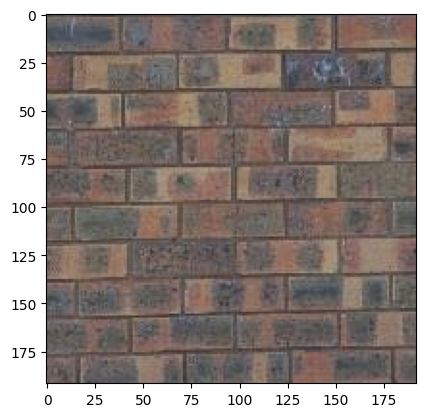
Perhaps the most naive texture synthesis algorithm is simply randomly sampling patches from the input texture image and stitching them together:
Parameters: (out_size, patch_size) = (400, 25)
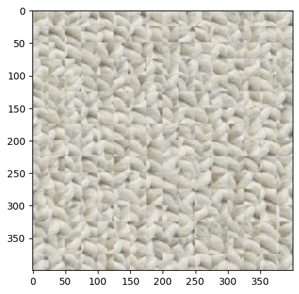
The results are unsatisfactory because there is no smooth transition between patches.
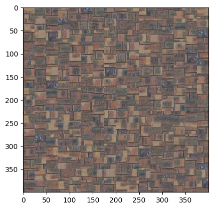
We can encourage smoother transitions between patches by making sure adjacent patches have similar overlap regions. This idea motivates the following algorithm:
tol patches and insert into the synthetic imageAs you can see, the edges are much smoother (though still not great):
Parameters: (out_size, patch_size, tol) = (400, 25, 3)
One futher optimization we can add to make the edges even smoother is defining a seam within the overlap region of the existing patch and the incoming sample patch. More specifically, for each sample patch we are inserting, we will compute a minimum cost path through the overlap region to find where pixels match the best, then leaving the existing texture on one side of the seam and inserting the incoming patch on the other side.
Here is the process in detail:

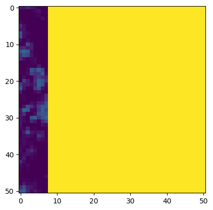
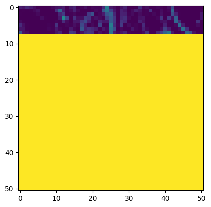
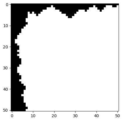
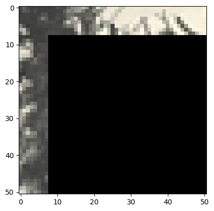
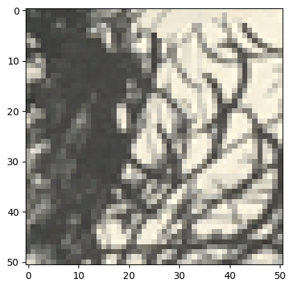
Our in-progress synthetic image has the first image patch, and we want to insert the second image. Let's compute SSD error in the overlap region:
We find a seam through these overlap regions where the error is minimized:
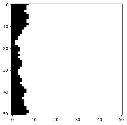
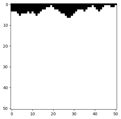
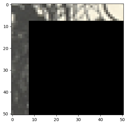
Now, we take the intersection of these masks to get our final seam. In the black region, we will keep the existing texture, and in the white region we will insert the incoming texture:
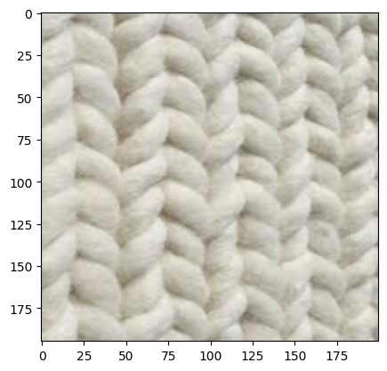
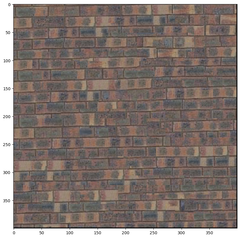
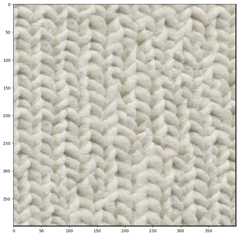
By doing this, we hope to smooth out the edges between adjacent patches. Here are the results using the same parameters as above:
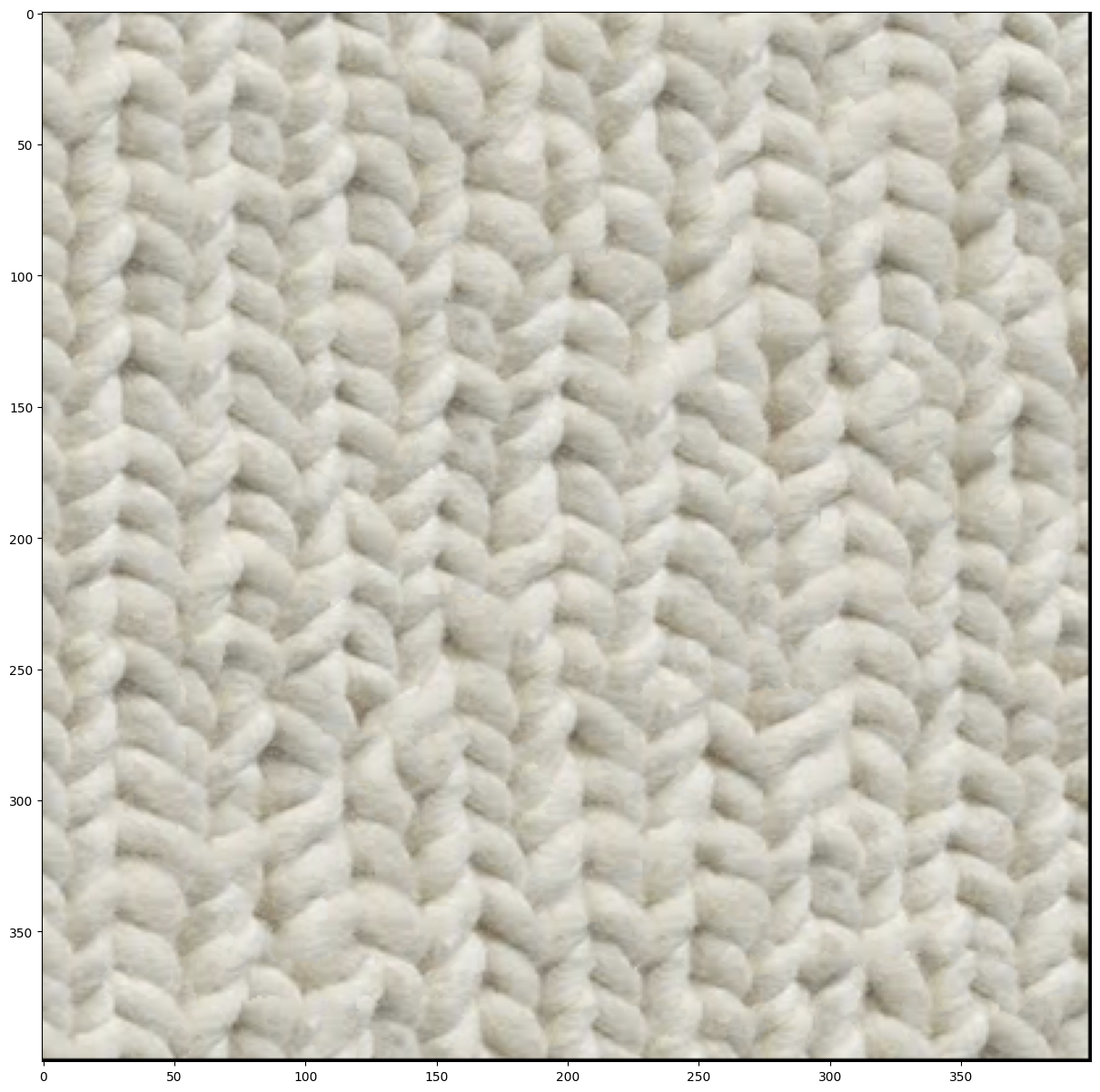
It is more obvious with the cloth texture, but in both it is harder to see the edges where each sample patch was inserted!
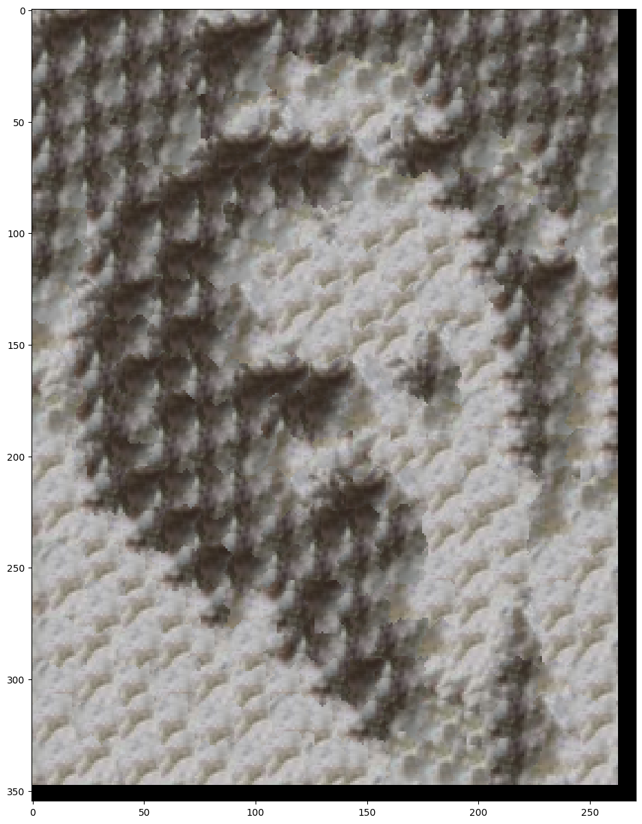
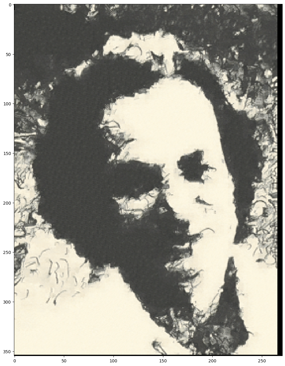
Now we will explore an interesting application of texture synthesis: transfering a texture onto an image! Essentially, our texture transfer algorithm augments our synthesis algorithm by requiring that each patch inserted satisfies a defined correspondence map in addition to the existing overlap constraints. Let's walk through an example:
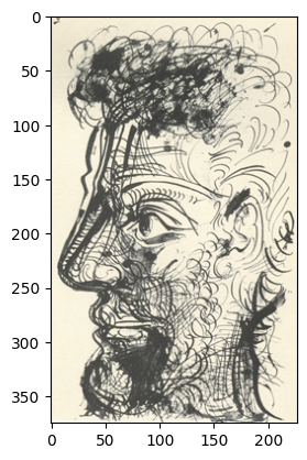
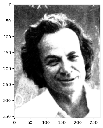
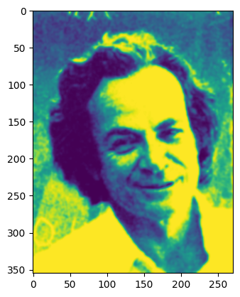
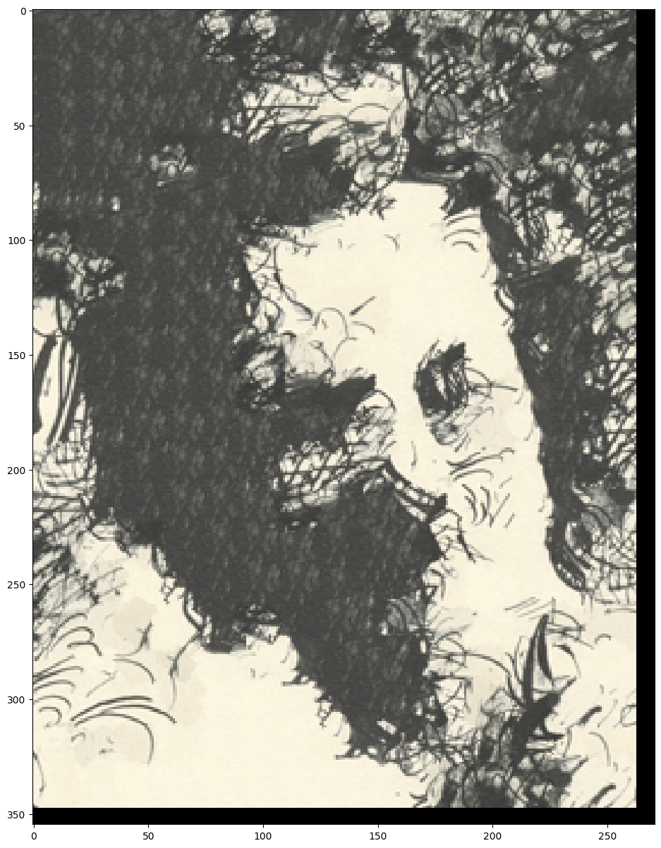
Here, we will try to recreate Feynman with the texture from the sketch. First, we will define correspondence maps, which are simply the result of applying some function to each image. Here, I used blurred luminance values for the sketch, and direct luminance values for Feynman:
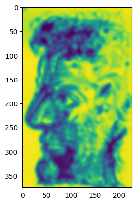
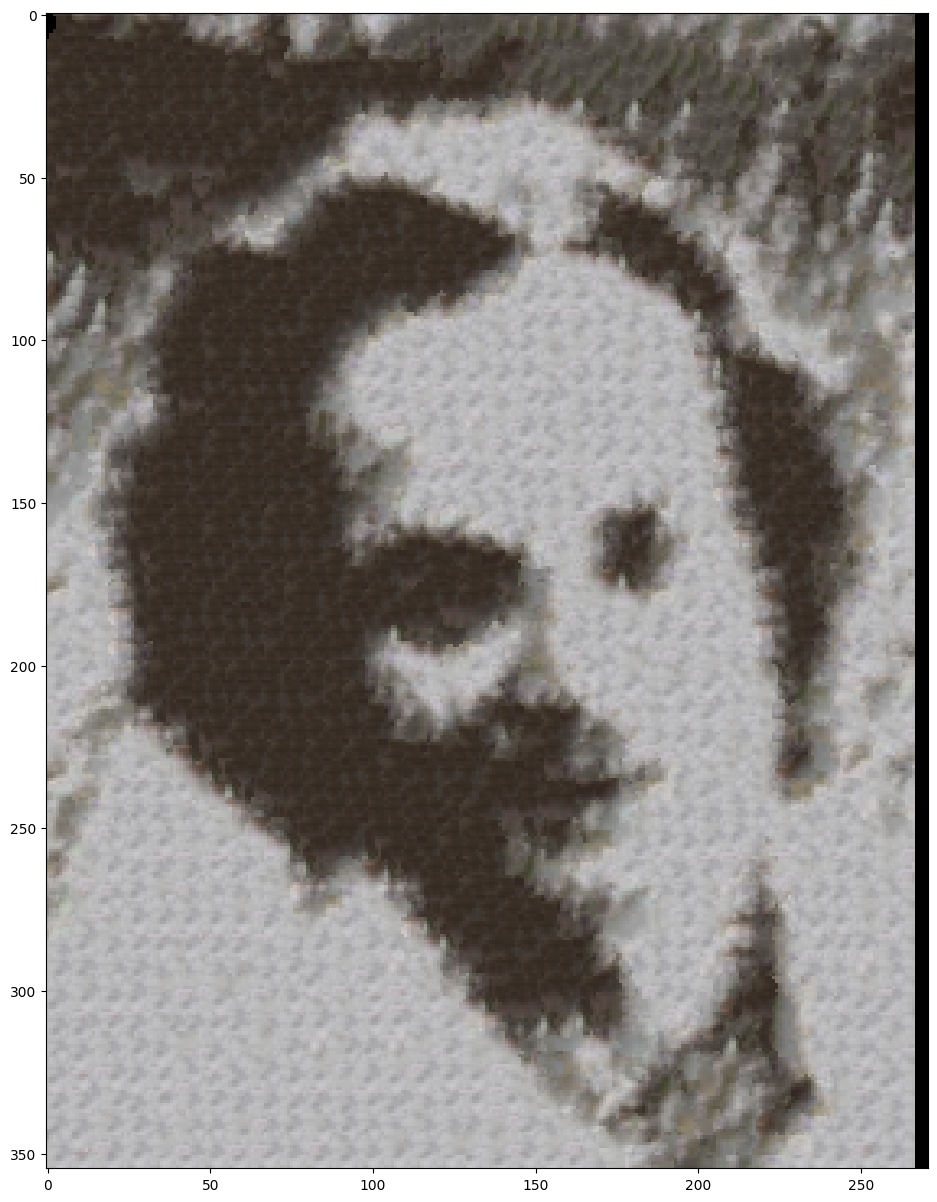
Then, as we are choosing a patch to insert, we modify the error term of the image quilting algorithm to be the weighted sum α times the block overlap matching error plus (1 - α) times the error between the correspondence map pixels within the source texture block and those at the current target image position.
Parameters: (patch_size, overlap, tol, alpha) = (25, 8, 3, 0.5)
Pretty cool! Here are some other results of texture transfer:
Since we only do one pass during the synthesis process, we are restricted to a single patch size and can lose detail. One optimization is to loop the texture synthesis process with gradually decreasing patch size. The only change from the non-iterative version is that in satisfying the local texture constraint, the blocks are matched not just with their neighbor blocks in the overlap regions but also with whatever was synthesized at this block in the previous iteration.
Also, we increase α each iteration according to the following formula: \( \alpha_i = 0.8 \cdot \frac{i - 1}{N - 1} + 0.1 \). This is so to make sure that as we progress, we still have good continuity behavior between patches and don't overfit to target image details.
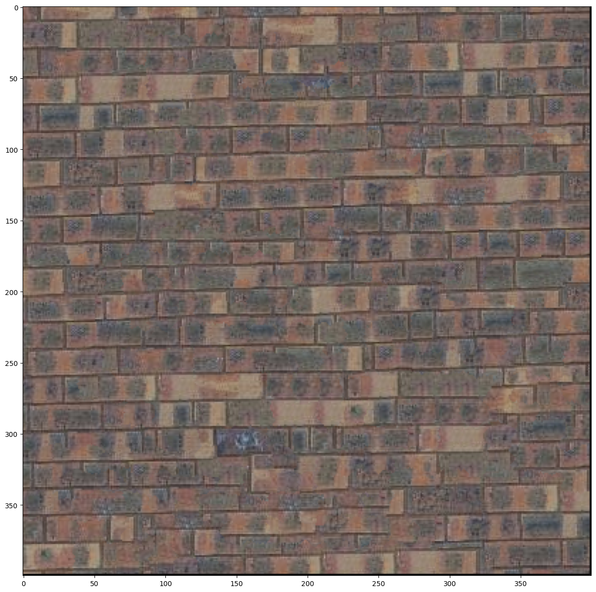
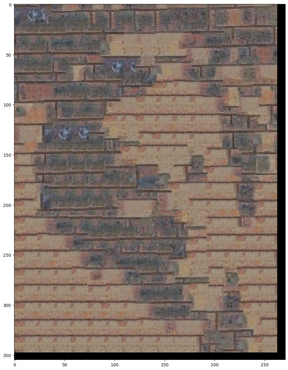
Parameters: (patch_size, overlap, tol, iterations) = (25, 4, 3, 4)
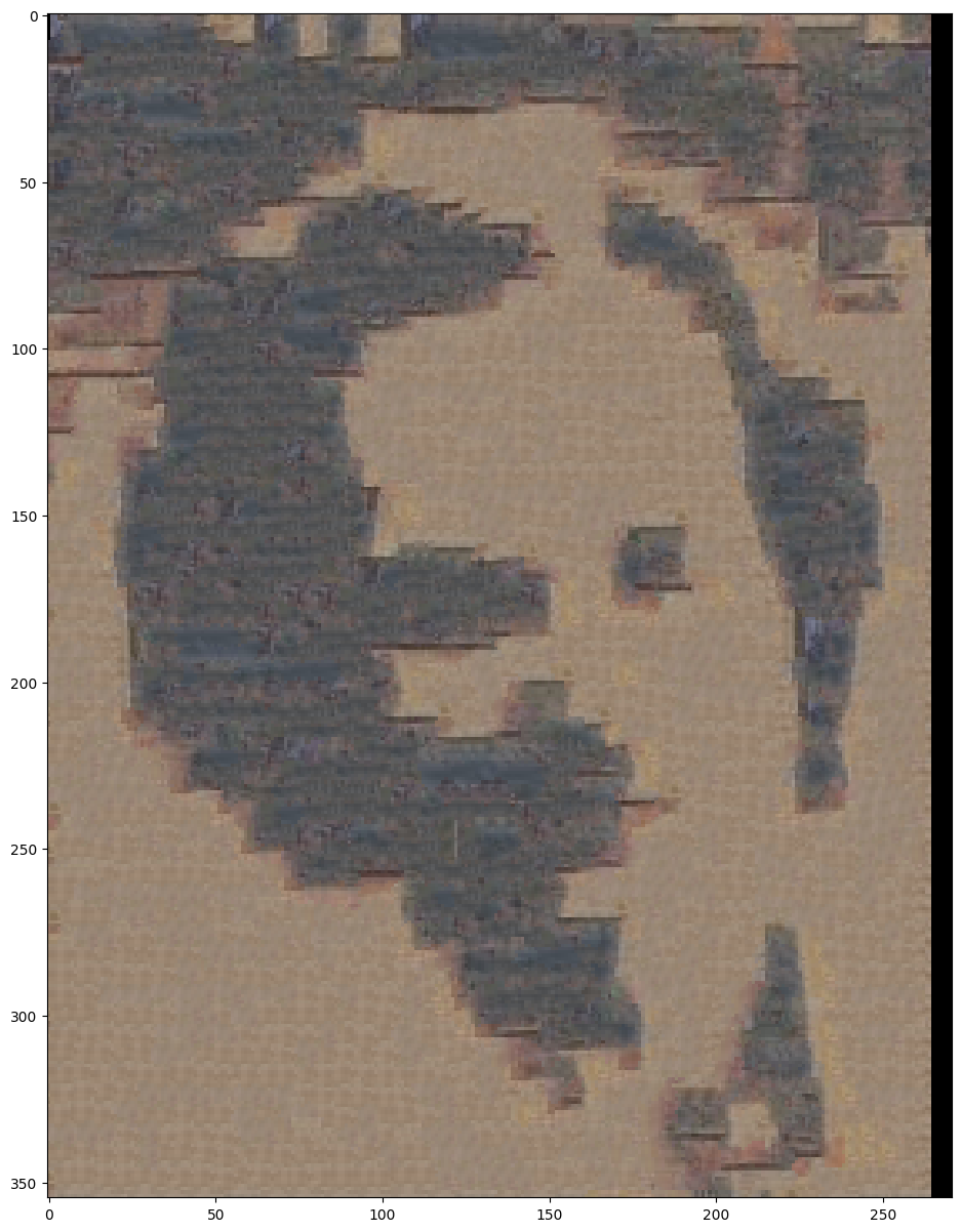
We can see that details, such as the mouth, are much more visible. However, as the patch sizes decrease, we also lose big picture structure and patterns, such as the brick pattern.
By Ethan Kuo
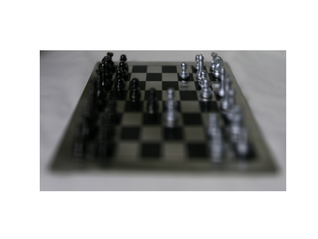
Using the chessboard images from the Stanford Light Field Archive, I first implemented depth refocusing. We have many images of the same chessboard that are taken from cameras shifted in the x, y directions. When we average these images, we see the back of the chessboard as clear while the front is blurry due to the parallax effect.
With the displacement of each camera from the center camera (x and y), I shifted each image by C * x and C * y. My findings show that when C is small (0), the front is blurry, while when C is big (3) the back is blurry.

Here is a GIF showing the chessboard from C=0 to C=3:
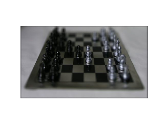
The previous part shows that C=1.5 is the best if we want the center of the chessboard clear. Now, we want to blur some of the outside of the chessboard. To do this, we ignore images that are more than a certain radius away from the center; this essentially acts as a camera aperture.
When R=0, we just get the center image. When R increases, we gradually average more images and thus get blurry results. The blur occurs on the borders because the new images we are adding are further and further away from the center image.


Here's the GIF from R=0 to R=8: