CS180 Project 5: Diffusion Models

By Ethan Kuo

Project 5A: The Power of Diffusion Models

Here, I played around with diffusion models, implemented diffusion sampling loops, and used them for other tasks such as inpainting and creating optical illusions

Part 0: Setup

Let's set up our pretrained model. Deepfloyd is a two stage diffusion model, where the first stage prduces an image of size 64×64 pixels, and the second stage produces an image of size 256×256 pixels. The model takes in a text prompt and outputs an image. When we sample from the model, we can vary the number of inference steps to take. Inference steps indicate how many denoising steps to take, with the a higher inference step correlating to higher image quality at the cost of computational cost. We also set a random seed to use for the rest of the project. We will be using the seed 1119. Below are some samples from the model given a prompt.

An oil painting of a snowy mountain village

There is noticeably more detail on the 100 inference steps images, such as texture on the snow and shadows on the houses.

A man wearing a hat

The generated image is a good match with the prompt. The diffusion model also added details that are not specified by the prompt, such as glasses and a woody backdrop. The stage 2 image looks just like a high resolution version of stage 1.

A rocket ship

Again the image is accurate based on the prompt. The model again took some creative liberties, such as making the rocket taking off rather than stationary.

Part 1: Sampling Loops

1.1: Forward process

In the forward process, we take a clean image $ x_0 $, and add noise to the clean image to get a noisy image $ x_t $ at timestep $ t $. The noise is sampled from a Gaussian distribution with mean $ \sqrt{\overline{\alpha}_t}x_0 $ and variance $ (1 - \overline{\alpha}_t) $.

Here, $ \overline{\alpha}_t$ is 1 when t = 0 and 0 when t is large.

This is equivalent to:

$ x_t = \sqrt{\overline{\alpha}_t}x_0 + \sqrt{1 - \overline{\alpha}_t}\epsilon $ where $ \epsilon \sim \mathcal{N}(0, 1) $.

1.2: Classical denoising

We will attempt to denoise these images using a Gaussian blur.

The results are unsatisfactory.

1.3: One-step denoising

Deepfloyd also has a UNet, a CNN that can predict Gaussian noise from a noisy image. We will pass the noisy images, a null prompt, and timestep t into this model to recover $ \epsilon $, then recover the initial image by solving

\[ x_0 = \frac{x_t - \sqrt{1 - \overline{\alpha}_t} \epsilon}{\sqrt{\overline{\alpha}_t}} \]

The results are much better, but the noisier the image was, the farther the recovered image strays from the actual image. For example, the last one looks almost cylindrical when the actual campanile is rectangular.

1.4: Iterative denoising

Diffusion models are trained to denoise across many steps. Here, we will use strided timesteps to denoise from t = 990, 960, ..., 0

We transition from the noisy image at timestep $t$ ($x_t$) to the noisy image at an earlier timestep $t'$ ($x_{t'}$), using the formula:

$$ x_{t'} = \frac{\sqrt{\overline{\alpha}_{t'}}\beta_{t'}}{1 - \overline{\alpha}_{t}}x_0 + \frac{\sqrt{\alpha_t}(1 - \overline{\alpha}_{t'})}{1 - \overline{\alpha}_{t}}x_t + v_{\sigma} $$

$x_t$ is our noisy image at timestep $t$.
$x_{t'}$ is our noisy image at timestep $t'$, such that $t' < t$.
$x_0$ is the one-step denoised version of $x_t$.
$\alpha_t = \frac{\overline{\alpha}_{t'}}{\overline{\alpha}_t}$.
$\beta_t = 1 - \alpha_t$.
$v_\sigma$ is random noise predicted by the DeepFloyd model.

Intuitively, we are incorporating information from each one-step denoised estimate, slowly approaching a clean estimate. Here are the results of iterative denoising the campanile, contrasted with one-step and Gaussian denoising.

Comparing these outcomes, I would say the iteratively denoised campanile is slightly better than the one-step denoised campanile since there is more detail. Gaussian denoising remains a poor option.

1.5: Diffusion model sampling

In the previous part, we went from a super noisy image of the campanile (basically indistinguishable from pure noise) into a clean version of the campanile. This begs the question: what happens if we iteratively denoise pure noise? Here are the results on 5 random noise samples with the general prompt "a high quality photo":

These are (mostly) coherent images, and the topic is completely random as expected.

1.6: Classifier free guidance

To improve the image quality at the expense of image diversity, we can use a technique called classifier free guidance. Given a noisy image, CFG combines a noise estimate conditioned on a text prompt $ \epsilon_c $ and an unconditioned noise estimate $ \epsilon_u $ to produce an overall noise estimate $ \epsilon $

$$ \epsilon = \epsilon_u + \gamma (\epsilon_c - \epsilon_u) $$

When $ \gamma $ is 0, $ \epsilon $ is the unconditioned noise estimate, and when $ \gamma $ is 1, $ \epsilon $ is the conditioned noise estimate. Interestingly enough, when $ \gamma > 1$ we get the highest quality images!

Again, here are 5 sampled images with the general prompt "a high quality photo":

I would say the CFG images are higher quality and more natural looking.

1.7: Image-to-image translation

Let's make edits to an image by adding some noise then forcing it back into the image manifold without any conditioning. Essentially, this forces the diffusion model to be "creative" in bringing a noisy image back into a "natural" looking image.

Here, we will add varying amount of noise to the campanile image (decreasing noise), then run CFG denoising to get an image "translated" from the original.

As expected, the more noise we introduce, the greater the edit since we are straying farther from the original image. At the extremes, we completely lose sight on the original topic.

1.7.1: Editing hand-drawn and web images

Can we make realistic versions of drawn images using image translation? Specifically, by adding some noise to a drawing then projecting it into the natural image manifold. Let's see:

Honestly, I'm a bit disapointed in these results. It seems that when we add just a little noise, there isn't enough room for creativity for the model to stray from the drawing and to make it look realistic. On the contrary, when we add too much noise, we lose sight of the meaning of the intial drawing.

1.7.2: Inpainting

Inpainting is the process of regenerating a specific part of an image. The inpainting procedure takes in an image $ x_{\text{orig}} $ and a binary mask $ \text{m} $, and creates a new image where $ \text{m} = 1 $, while keeping the original image where $ \text{m} = 0 $.

The inpainting algorithm denoises pure noise using CFG but with one simple modification: after obtaining $ x_{t'} $ in each iteration, we "force" $ x_{t'} $ to have the same pixels as $ x_{\text{orig}} $ where $ \text{m} = 0 $ through the equation:

\[ x_{t'} \leftarrow \text{m} x_{t'} + (1 - \text{m}) \cdot f(x_{\text{orig}}, t') \]

where $ f $ is the forward process from earlier. Here, we apply inpainting to the top of the campanile:

The results are... interesting. It is quite funny how a baby was inpainted on the minigolf hill, and I thought the black cat on a tree branch with the moon in the background was very creative! One thing to note here is that the diffusion model is generating a pure projection to the natural image manifold, which makes sense given the random results. In the next part, we will add a text prompt to guide image generation.

1.7.3: Text conditioned image-to-image generation

Here, we are generating images off the campanile image with the prompt "a rocket ship". As expected, the more noise we introduce, the less campanile-like the result it is, and we can always see something like a rocket ship.

1.8: Visual Anagrams

A visual anagram is essentially an optical illusion. In this part, we will create an image that looks like one thing, but when flipped upside down will reveal another thing

To do this, we will use CFG but set the noise estimate for each iteration to be an average of both prompts. Specifically, we denoise an image $x_t$ at step $t$ normally with the first prompt to obtain noise estimate $\epsilon_1$. But at the same time, we will flip $x_t$ upside down, and denoise with the second prompt to get noise estimate $\epsilon_2$. We can flip $\epsilon_2$ back, to make it right-side up, and average the two noise estimates. We can then perform a reverse diffusion step with the averaged noise estimate.

The noise estimate formula is: \[ \epsilon_1 = \text{UNet}(x_t, t, p_1) \] \[ \epsilon_2 = \text{flip}(\text{UNet}(\text{flip}(x_t), t, p_2)) \] \[ \epsilon = \frac{\epsilon_1 + \epsilon_2}{2} \]

Here are some results!

An oil painting of people around a campfire

An oil painting of a post-apocalyptic city

1.9: Hybrid Images

Just like in project 2, we will create images that appear differently up close and afar. Similar to visual analogs, we employ CFG but with a modified noise estimate formula. Here, we estimate the noise based on both prompts then combine the low frequencies of the first image with the high frequencies of the second image.

The noise estiamte formula is: \[ \epsilon_1 = \text{UNet}(x_t, t, p_1) \] \[ \epsilon_2 = \text{UNet}(x_t, t, p_2) \] \[ \epsilon = f_{\text{lowpass}}(\epsilon_1) + f_{\text{highpass}}(\epsilon_2) \]

I am impressed by how good these hybrid images are! They are much better than the results I had from Project 2, where I manually picked 2 images to make a hybrid.

Part B: Diffusion Models from Scratch

Here, we will create a diffusion model from scratch using the MNIST dataset. We'll create a generative model capable of synthesizing images of handwritten digits similar to those in the MNIST dataset.

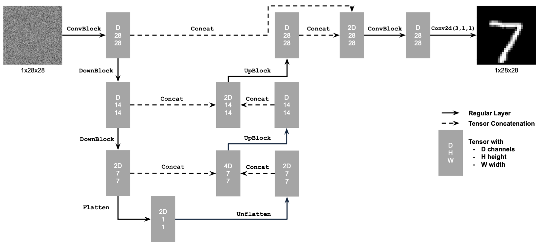
Part 1: Training a Single-step Denoising UNet

1.1: Implementing the UNet

As we know from the previous part, a UNet takes in a noisy image and outputs a noise estimate, which we can subtract to get a cleaner image. Here, we use torch.nn to create a class UnconditionalUnet(nn.Module) with a forward(x) function that implements the following neural network:

1.2 Using the UNet to Train a Denoiser

To train this model, we will use the MNIST dataset, which consists of many images of handwritten digits. The training data is in the format $ (z, x) $, where $ x $ is the image and $z = x + \sigma \epsilon \quad \text{where} \ \epsilon \sim \mathcal{N}(0, I) $. Essentially, $ z $ is a noisy version of $ x $. We will train our model parameters using the L2 loss function $L = \| D_\theta(z) - x \|^2 $.

While preparing the training data, I added various levels of noise to the digits to visualize the forward process. Ultimately, our diffusion model will do the reverse process, taking pure noise and moving towards a handwritten digit incrementally.

1.2.1 Training

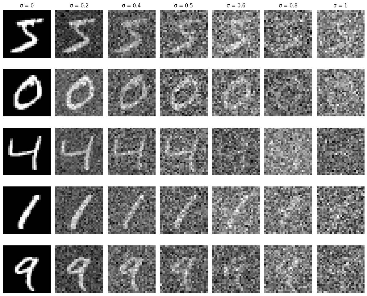
I trained the model using the following hyperparameters:

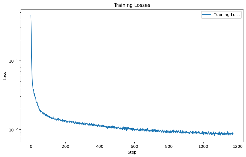
epochs = 5
batch_size = 256
learning_rate = 1e-4
D = 128

Also, I used the Adam optimizer for its speed, and I trained the model with noisy images with $ \sigma = 0.5 $ paired with the original image.

The training results are shown in the loss curve:

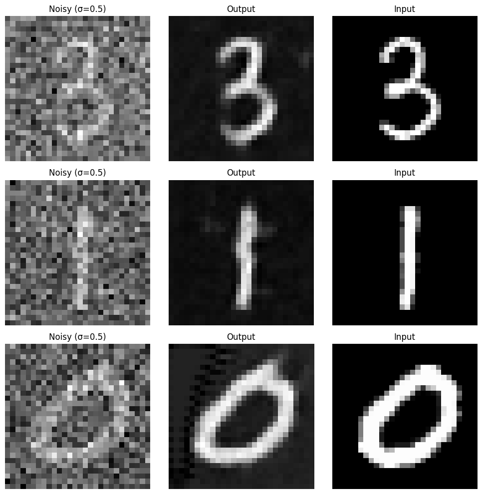
By looking at how our model performs on unseen test data in the first and last epoch, we can see that as the model is improving:

1.2.2 Out-of-Distribution Testing

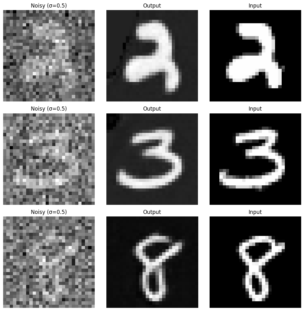
Even though the model was trained on images noised with a variance of 0.5, it can still be used on images with different noise levels. Here is how the model performs on random test set data with varying noise levels:

Results are worse as there is more noise, but we can see that the performance is still pretty good! Our model is definitely capable of denoising a reasonably noisy handwritten digit. Awesome!

However, our model would not be capable of generatoring legitimate images of handwritten digits from pure noise, as shown by the poor results with high noise levels. Can we do better?

Part 2: Training a Diffusion Model

We want a diffusion model to be performant for any noise level $t = 1, ... , T $. A naive solution is to simply build T UNets as in Part 1, training each on images with a specific noise level. A better solution is to implement a single UNet with time conditioning that can accurately estimate noise for any noise level. Then, we can use the iterative denoising algorithms we've discussed in Part A to arrive at a clean image.

2.1 Adding Time Conditioning to UNet

Implementing this UNet is extremely similar to the previous one. One small difference is that we can change our UNet to predict the added noise instead of the clean image. Another is that we will embed the timestep into our existing model using FCBlocks.

2.2 Training the UNet

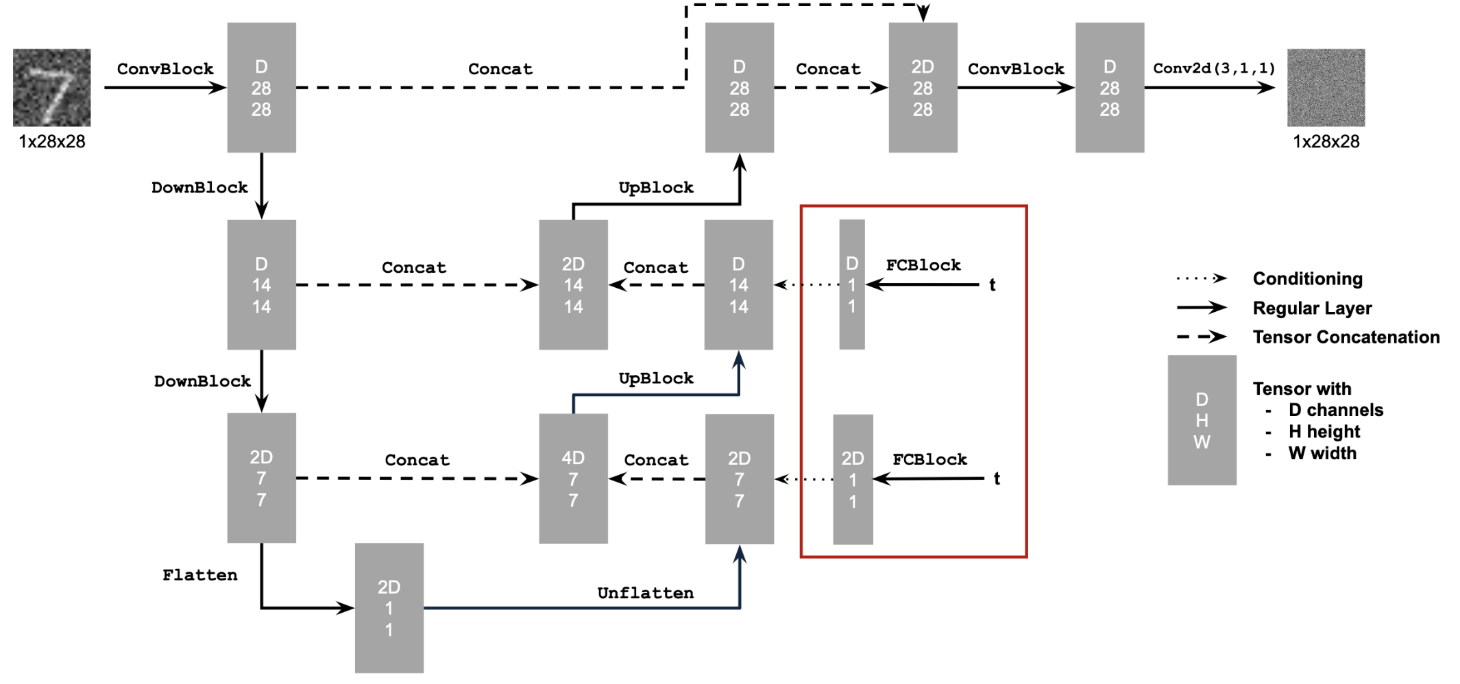
We train the model on images of various noise levels until satisfaction.

I trained the model using the following hyperparameters:

epochs = 20
batch_size = 128
learning_rate = 1e-3 with exponential learning rate decay of $ \gamma = 0.1^{\left(1.0/\text{epochs}\right)} $
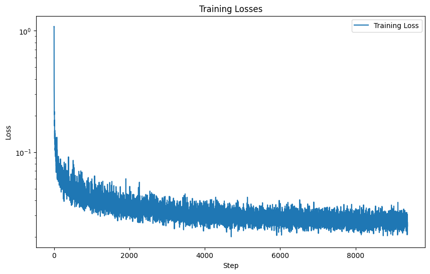
D = 64

Also, I used the Adam optimizer for its speed. The training results are shown in the loss curve:

2.3 Sampling from the UNet

Now that our model is trained, let's sample some images! More precisely, we will pass in pure noise into our model to produce a one-step denoised estimate, remove some noise using that estimate, then repeat the process across many timesteps.

Here are the results for the time-conditioned UNet for 5 and 20 epochs

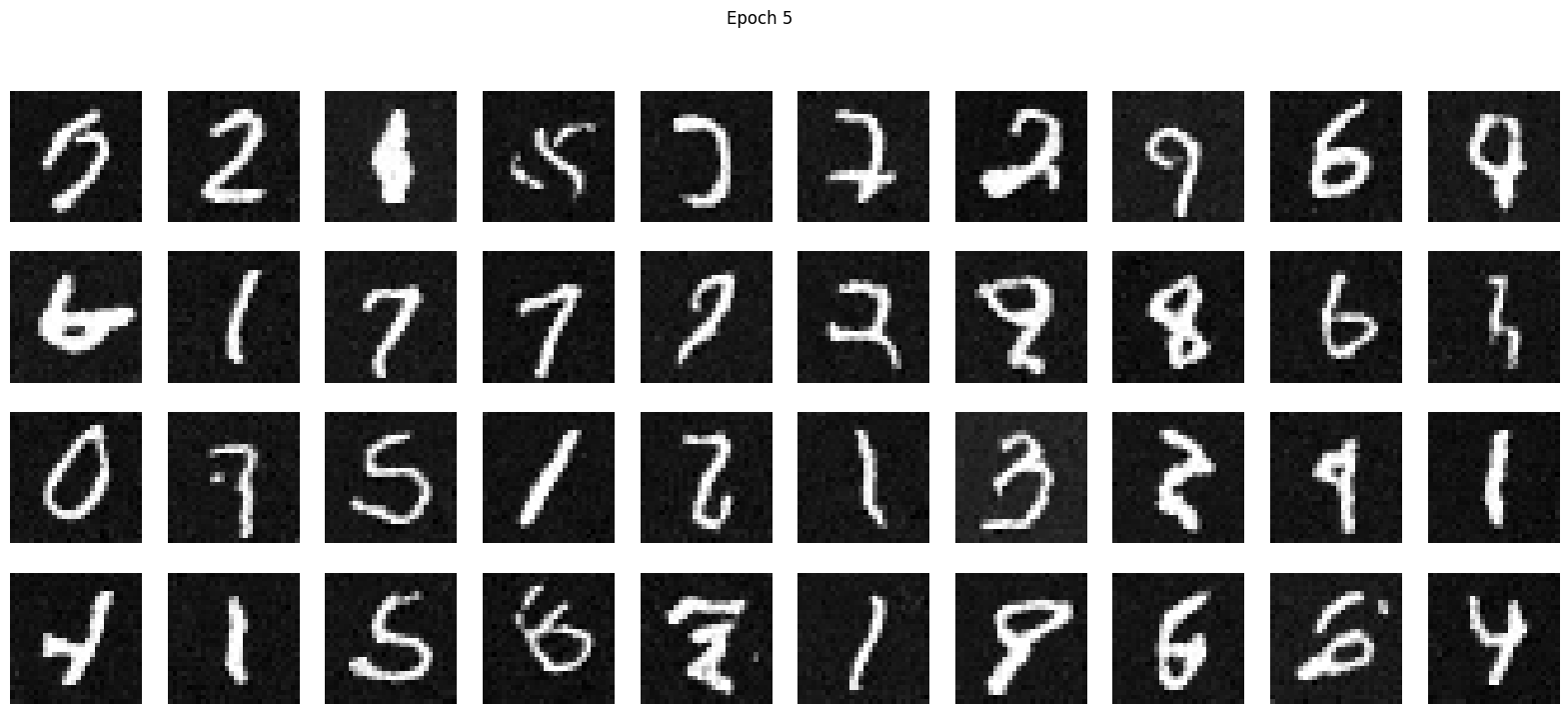
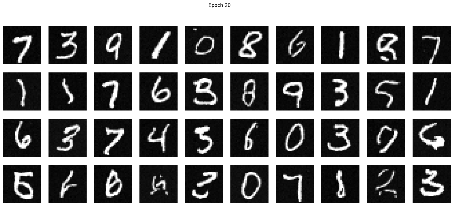
We can see that the longer we train for, the better quality the images are. However, some are still unintelligable.

2.4 Adding Class-Conditioning to UNet

What if we want to generate a specific digit? We will train the model with a class condition. Basically, our model will not only be trained by a noisy image and a timestep but also its true class (a number from 0 to 9). This class will be one hot encoded and then be passed into the model.

However, we still want our model to be able to work on unlabeled data, so we implement a 10% dropout so that some of our training data will not have its true label considered. Here is the training loss curve:

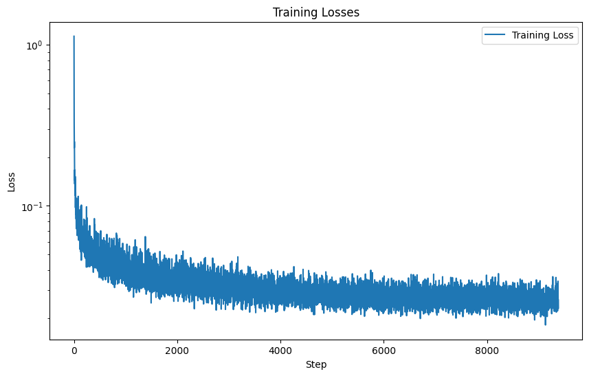
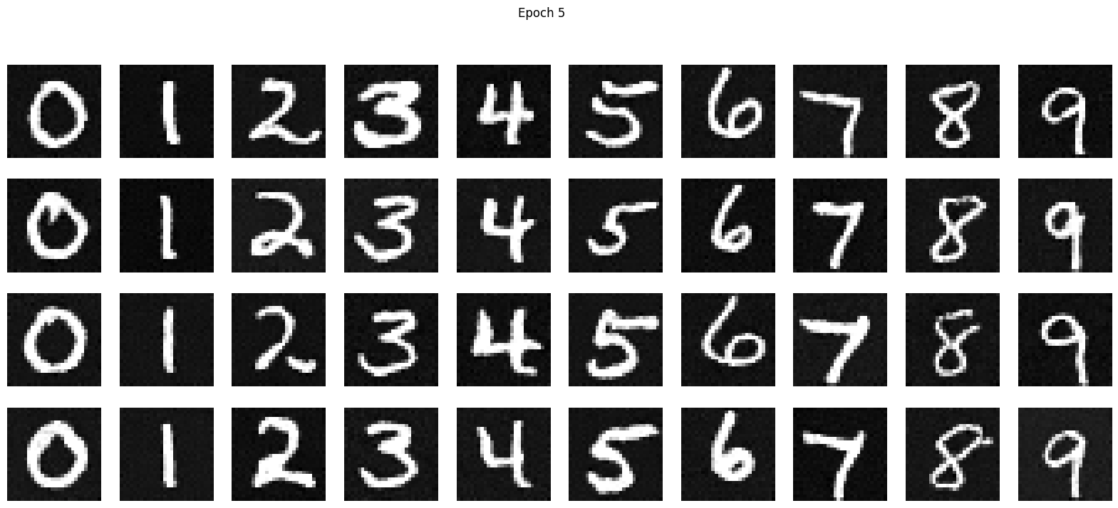
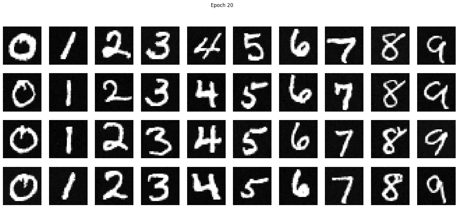
2.5 Sampling from the Class-Conditioned UNet

We know from Part A that classifier-free guidance allows for high quality image generation from pure noise, so we implement CFG here with $ \gamma = 5$, using our class-conditioned UNet to derive one-step noise estimates.

Here are the results for the time-conditioned UNet for 5 and 20 epochs

Conclusion

It was great to learn the workflow for implement a machine learning model from scratch. It's awesome that I've built a model that can generate images of any digit I want!