By Ethan Kuo
A mosaic in the context of image processing is an image created by seamlessly stitching together multiple images, usually to create a larger panoramic view or to blend two images into a single composite. In the first part of this project, we will create mosaics of 2 photos.
Here are the photos we will build mosaics from. Each pair of photos is taken from the same center of projection and has around 50% overlap.
A homography is a transformation that can change the perspective of 2 images captured from the same center of projection. This will be used to transform all images of a mosaic into the same point of view.
First, we need to define point correspondances between the two images.
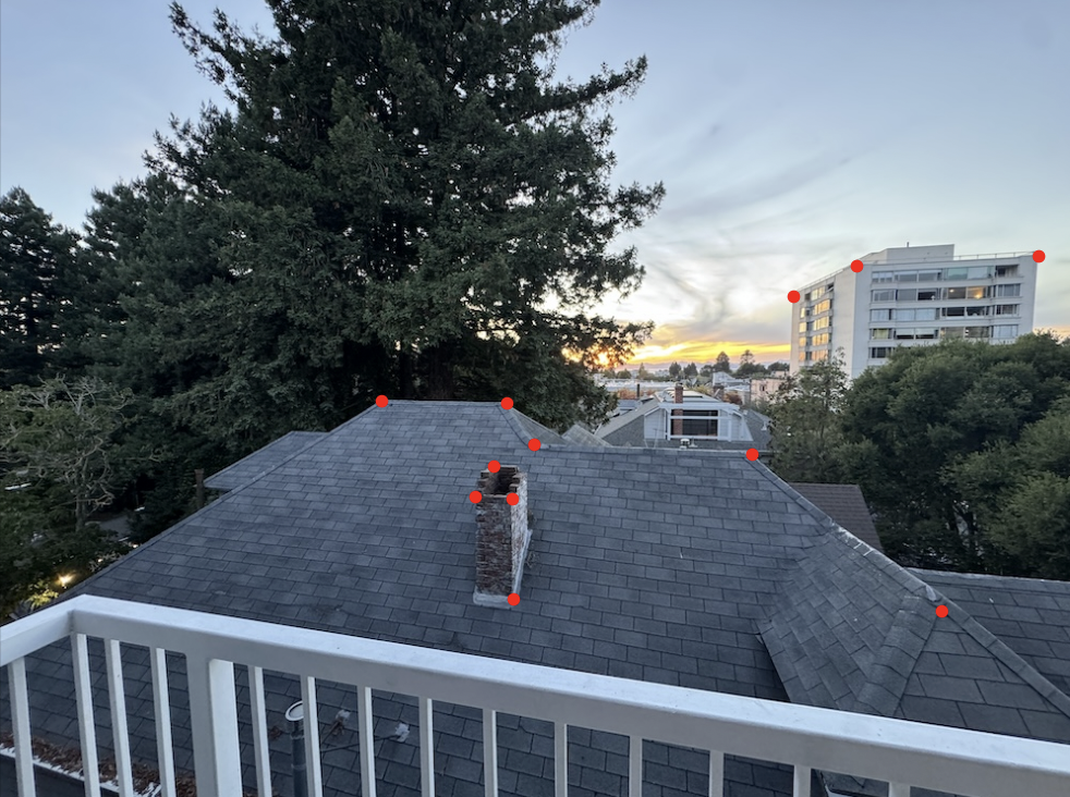
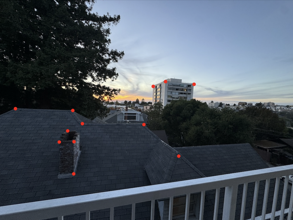
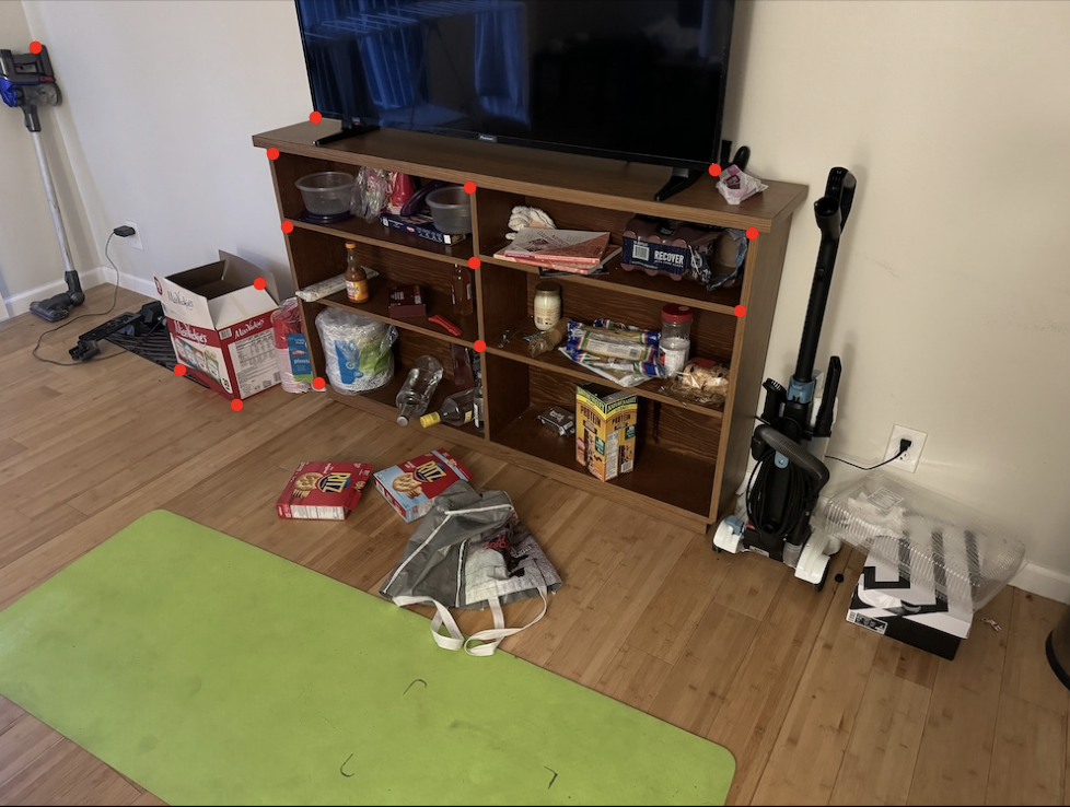
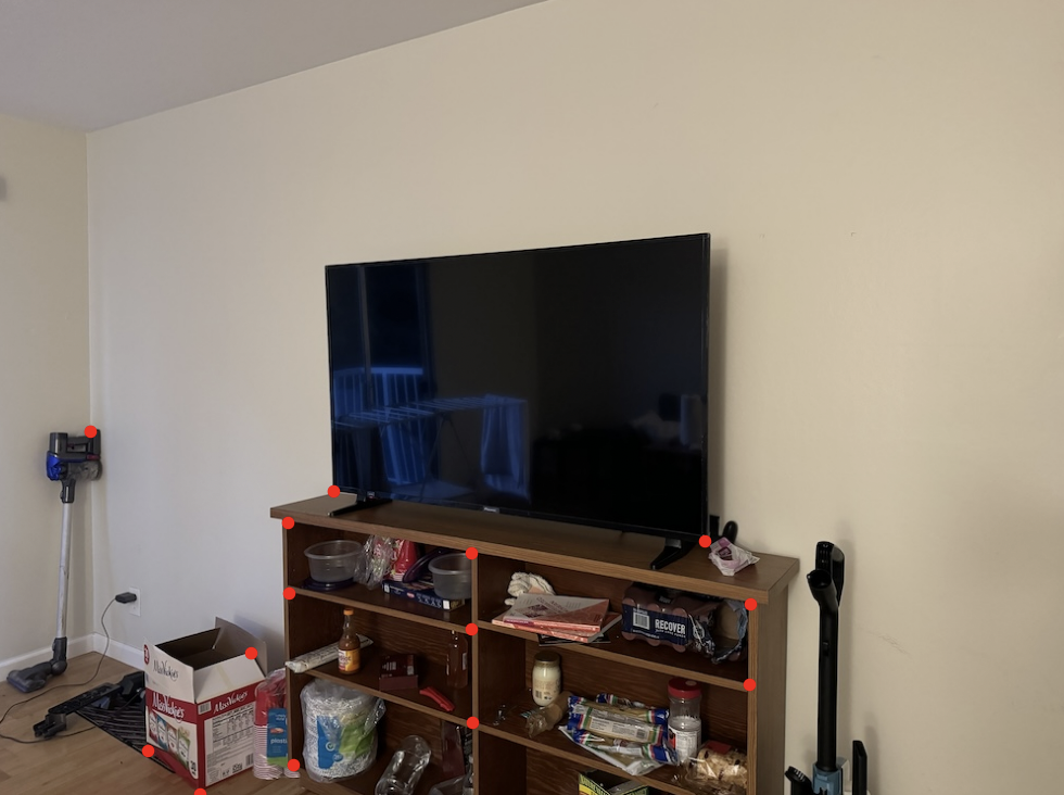
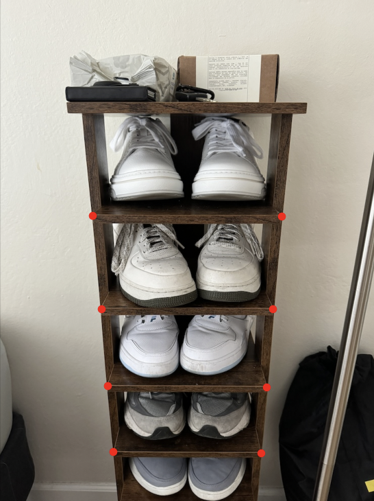
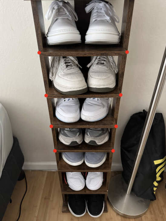
Next, we compute the 3x3 homography matrix that maps one set of points to the other. We want
to recover the matrix such that:
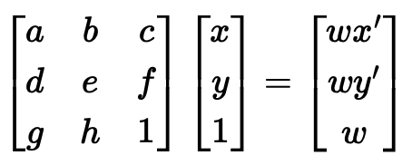
Expanding this out, we get the following system of 2 equations:
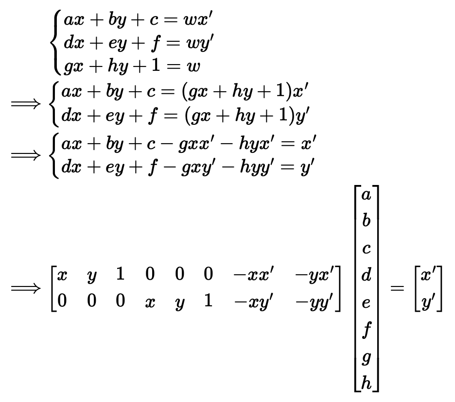
Note that there are 8 unknowns in the homography matrix, so technically we only need 4 point correspondances for a solution (each correspondance yields 2 equations). However, I picked more correspondances and then applied least squares to get a more stable solution.
Simplying applying the homography H to every point in an image will not suffice since we may get
holes in the warped image. So, I used inverse warping as in Project 3. First, I computed
the bounding box of the warped image by applying H to the four corners of the image. Then, I
applied the inverse of H to every point in the bounding box to "pull" the color for that pixel from
the preimage. Since homographies often produce an irregular bounding box shape, it is entirely possible for the
preimage to be outside
the source image; in these cases, we simply make that pixel black.
Let's demonstrate the warping algorithm with image rectification, or "straightening out" some part of an image into a rectangle. For example, each of these images has a rectangular component:
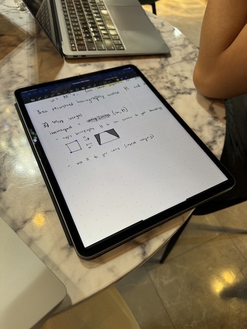
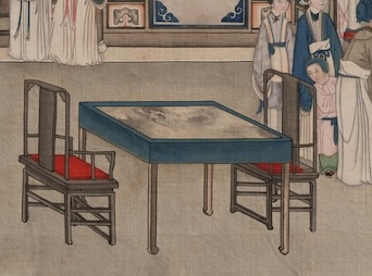
We compute the homography matrix that maps the corners of the rectangular object into a true dimensions of the
rectangular shape, such as [0,0], [1,0], [1,1], [0,1]. Then, we run the above warping algorithm.
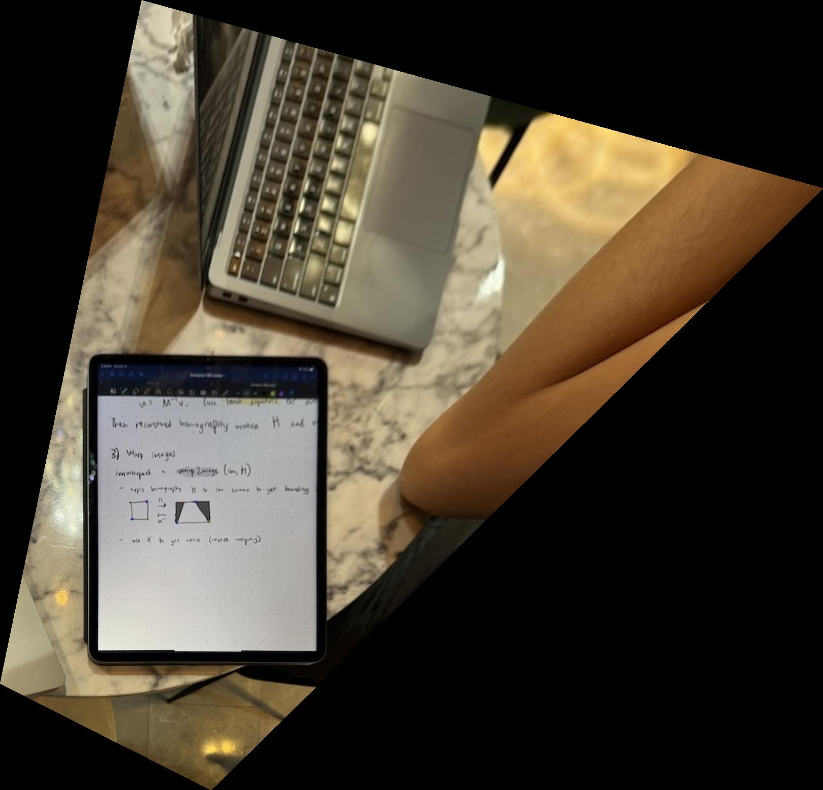
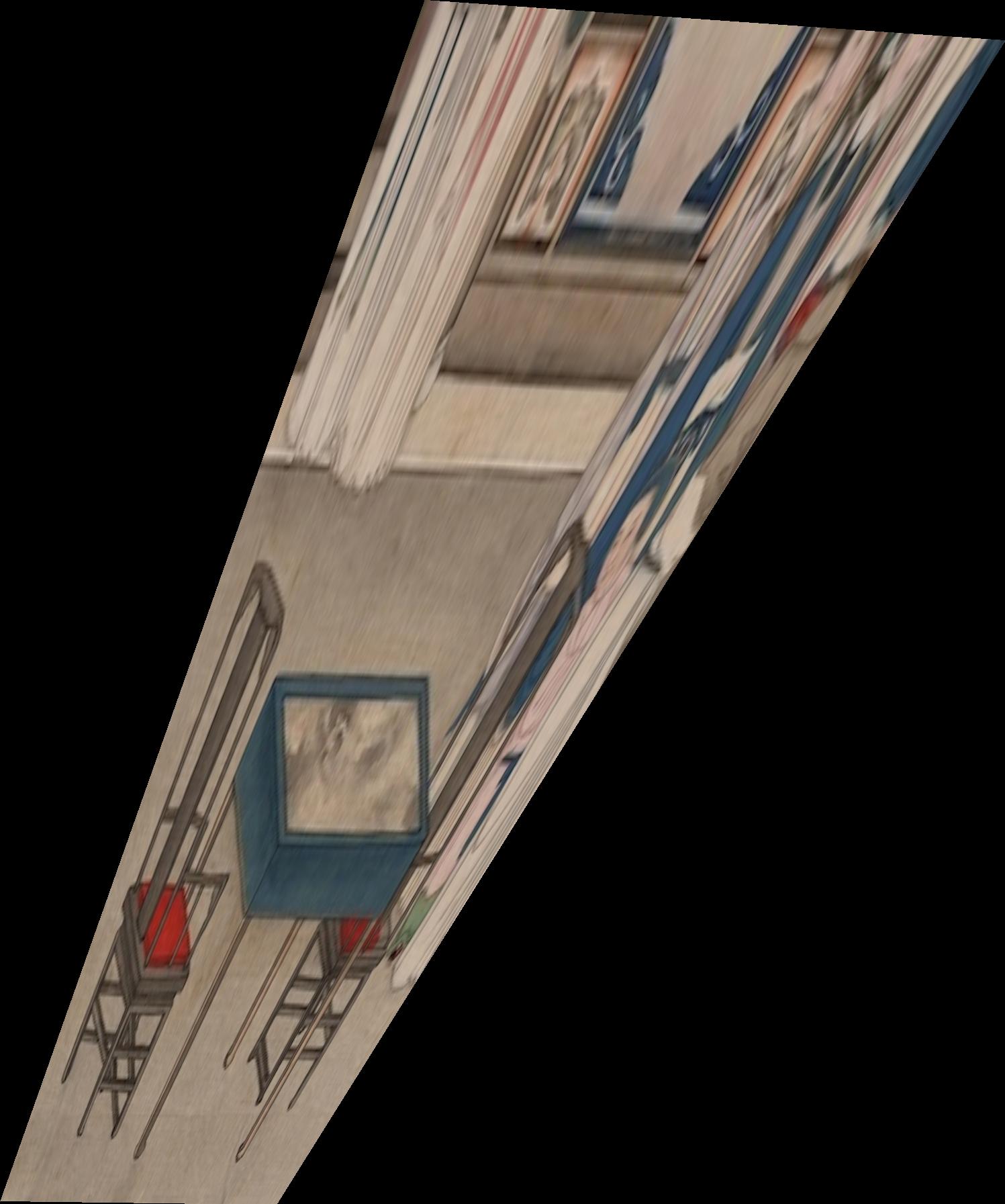
For 2-image mosaics, the simple approach I took is to warp the perspective of the second image into the first. Then, we align the first image with the warped second image and average the pixel values when there is overlap.
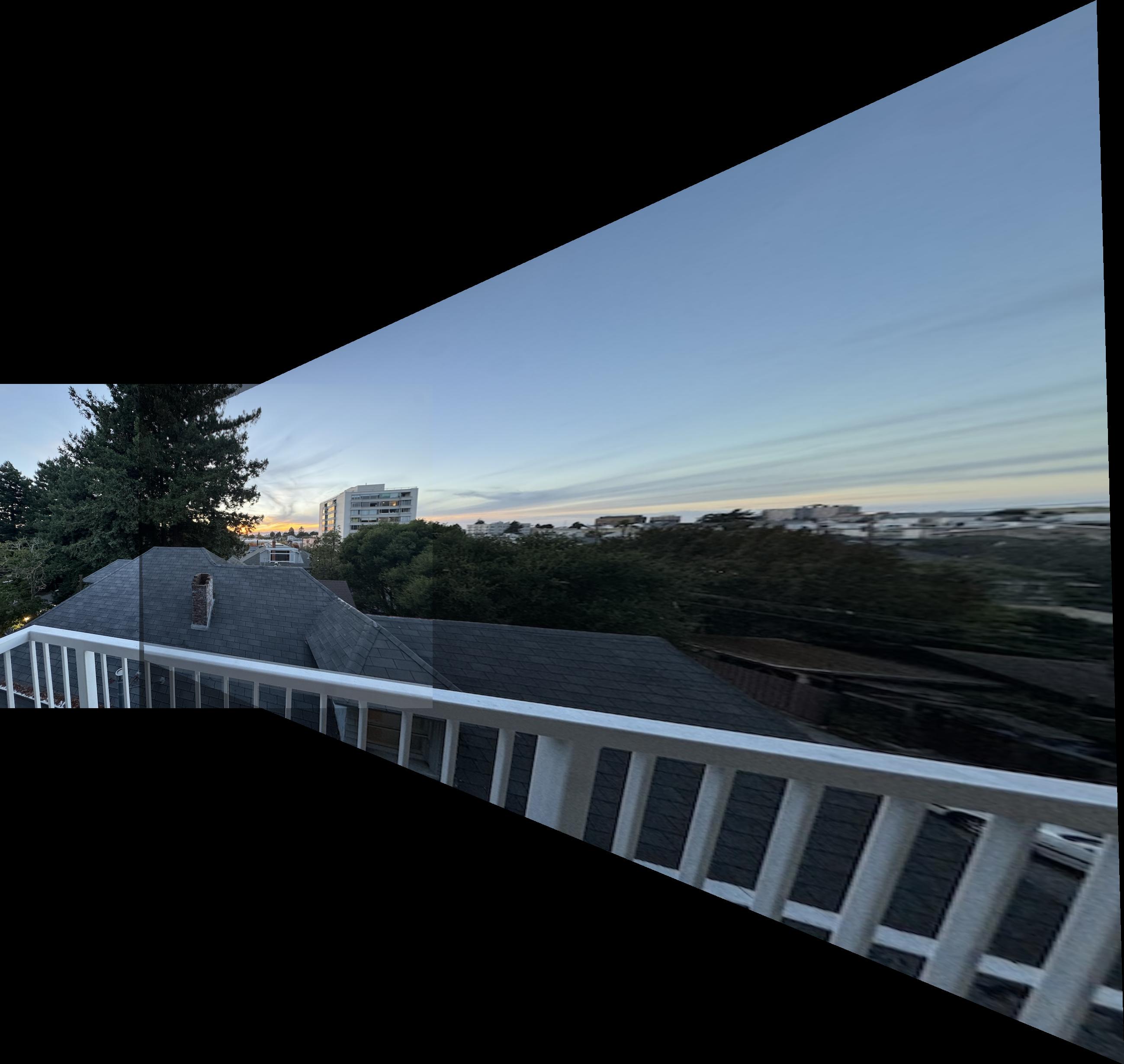

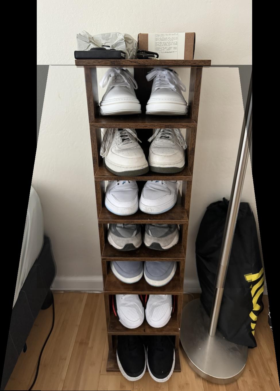
Note the edges where the overlap starts and ends. The photos may have different exposures, so simply averaging pixel intensities will result in stark changes.
I used two-band blending to make a more seamless transition. First, I computed the distance transform of each image, which is a mask that records the distance of each point to the nearest edge. Intuitively, an image's middle area is its focus and should we weighted higher, so the distance transform can be used as weights. Here are the distance transforms for the balcony images:
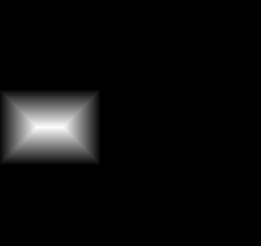
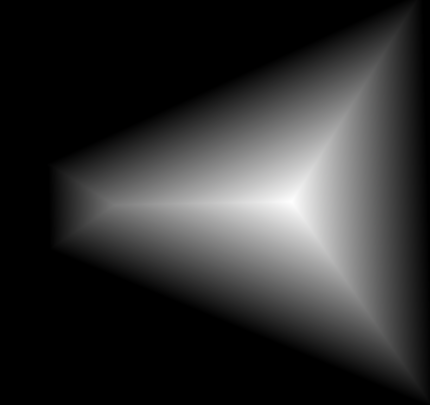
Then, we will blend the low and high frequencies separately, hence a "two-band" approach..
Lower frequencies capture big-picture information like backgrounds, so taking a simple weighted average makes sense. The low-pass images are blended according to a weighted linear combination of the two images using the distance transforms as weights.
Higher frequencies capture fine details in an image. Since the details in an image will likely be more accurate when they are in the center of the image, we will simply adopt the high frequencies from the more focused image. The high-pass images are blended depending on the maximum value of the corresponding distance transforms.
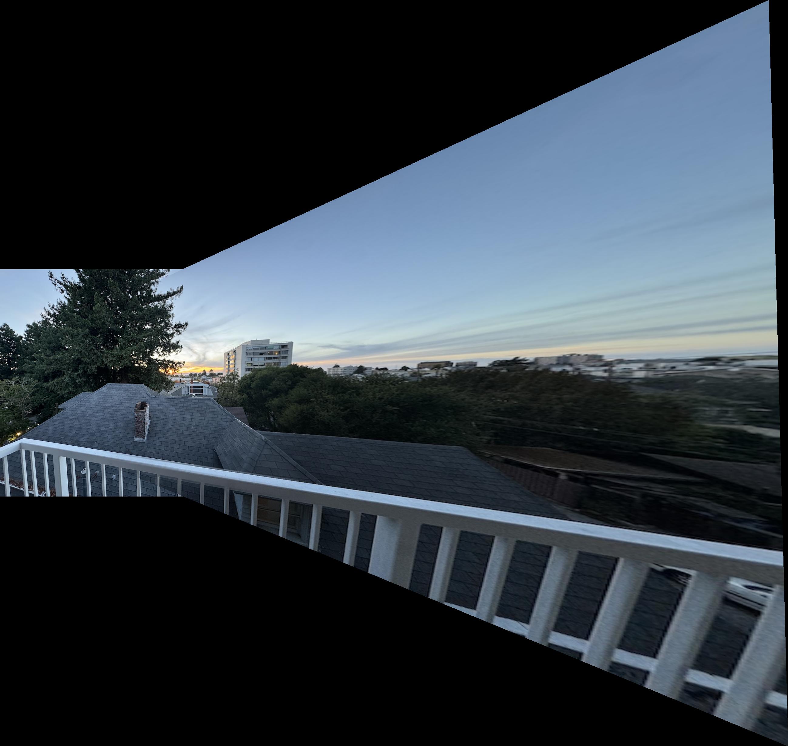
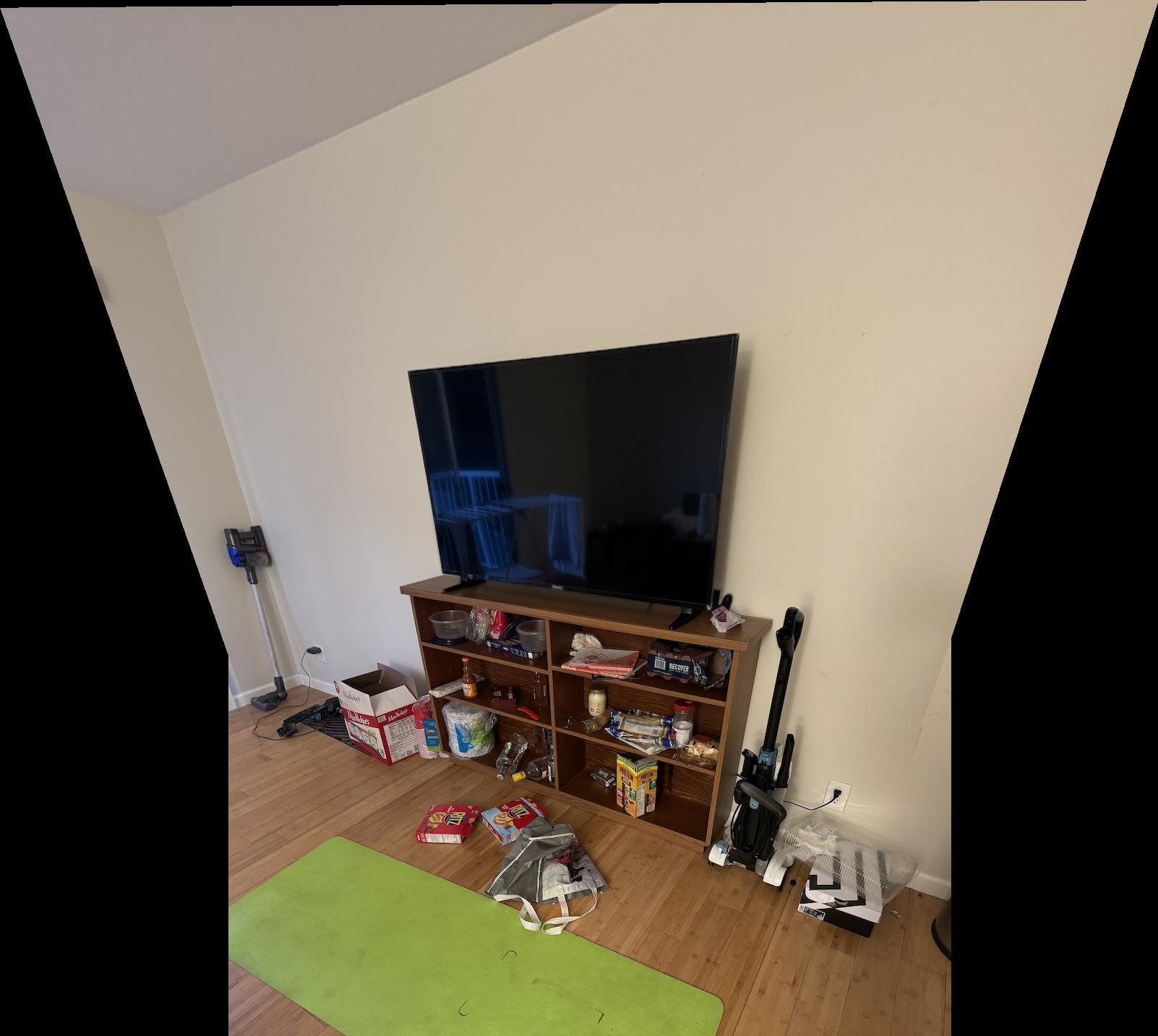
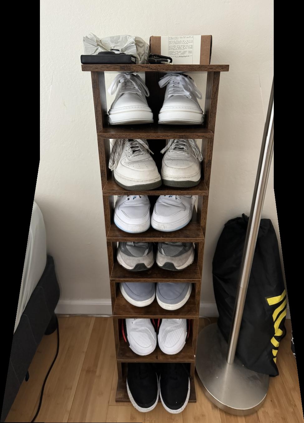
Here are the blended mosaics:
Previously, I had to manually choose correspondance points between two images. In this part, we will implement an algorithm for automatically defining correspondances. On a high level, our algorithm will consider "corners" in both images and match corners that have similar features.
Let's walk through the automatic feature matching algorithm on the balcony example.
The Harris corner detection algorithm finds corners an image. Without going into excess detail
on the linear algebra, the algorithm builds a 2x2 matrix out of the gradient, which captures how
much the pixel changes in all directions. Intuitively, a corner is a pixel that changes value significantly in
all
directions, so the algorithm gives a high corner response score for corners whose matrices have large
eigenvalues
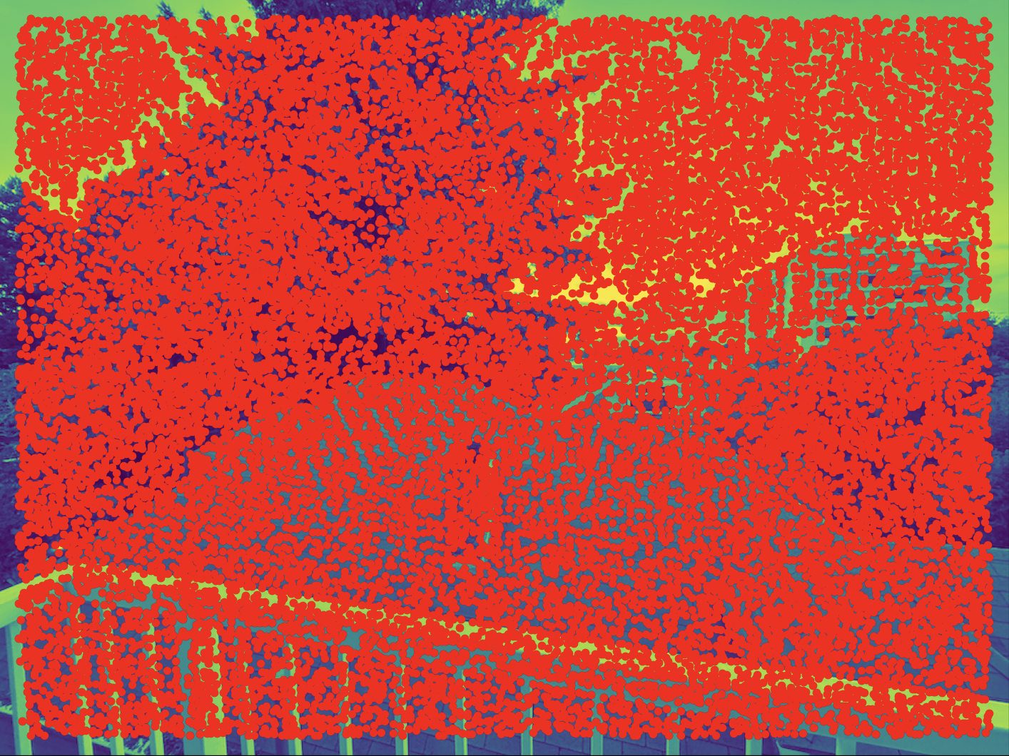
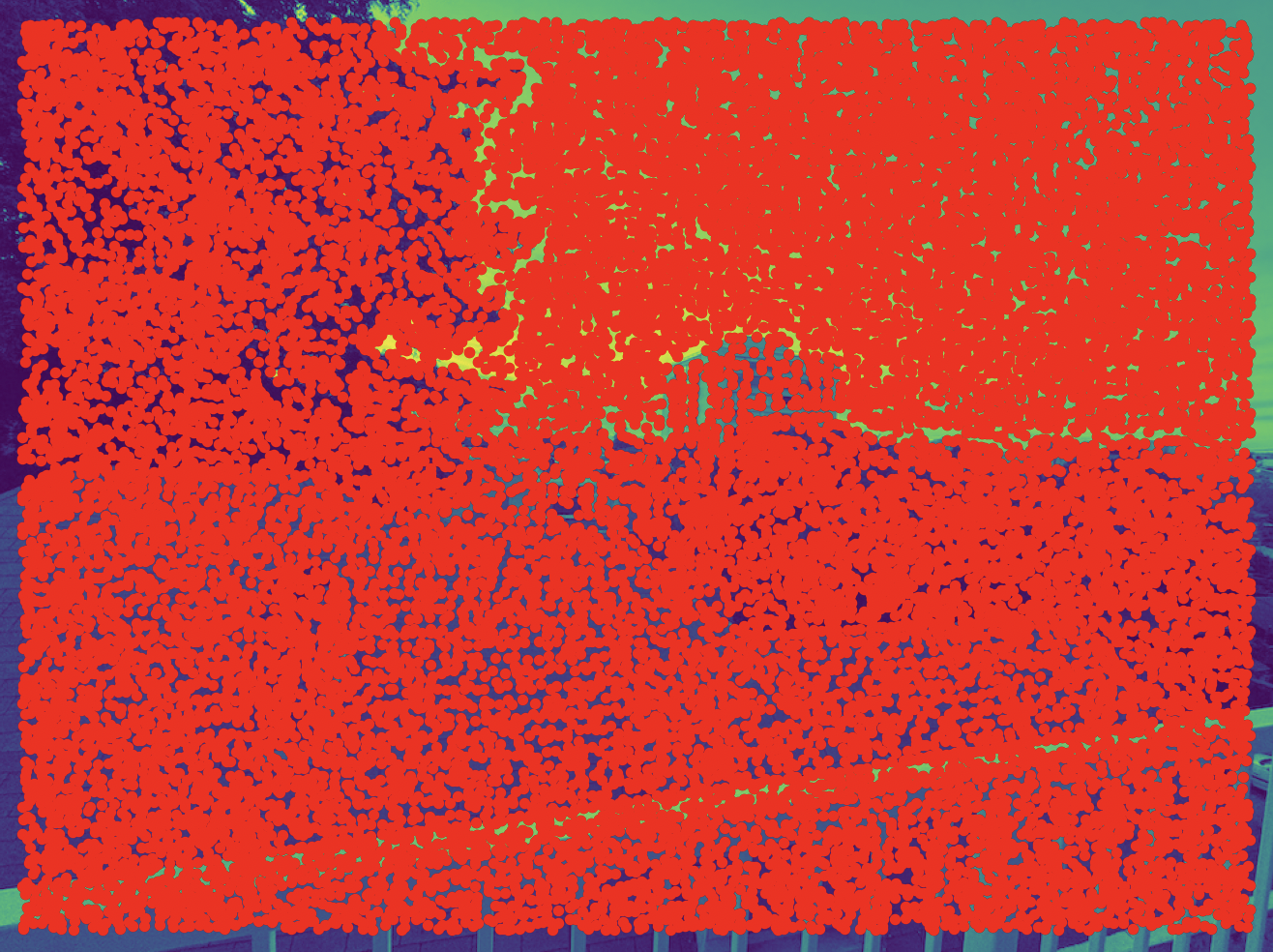
As you can see, there are many corners in an image, so we will need to narrow our search.
The ANMS algorithm takes in Harris corners and chooses corners that 1) have a high Harris response score and 2) are spatially distributed across the image. These are reasonable criteria because we want our keypoints to be actually "good" corners and to span most of the image.
For each candidate corner, ANMS finds all corners that are "better" than that corner by margin, then
computes the distance to the nearest one. Then, it outputs the top k corners with the greatest
distance. Note that strong corners are rewarded since there will be fewer better corners it computes its
distance from, and corners distant from other corners are clearly rewarded. So this objective encodes the
criteria from above.

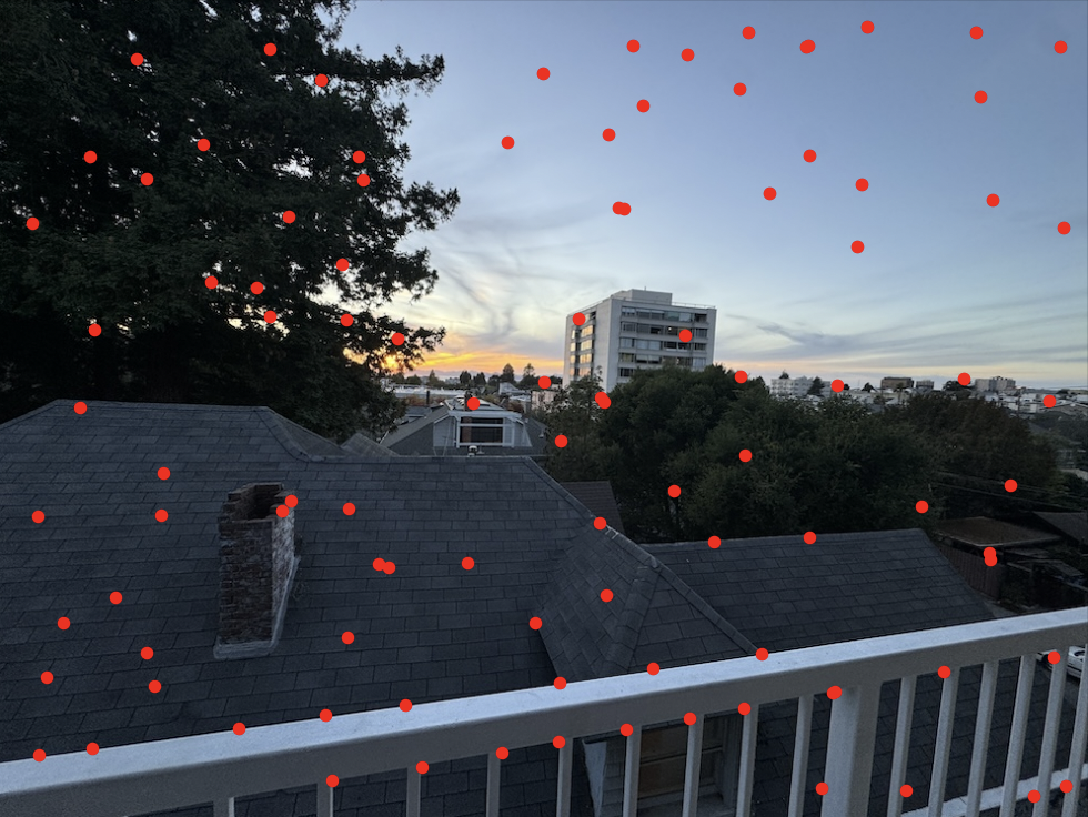
Now that we have points in both images, we want to match points that have similar features.
We'll start by defining these features by looking at the point's vicinity. First, we will apply a low-pass
filter over each image. Next, for each
point, we take the
40x40 patch around the point, downsample it into an 8x8 patch (which observes minimal
aliasing
due to the low-pass filter), then normalize the patch to have a mean of 0 and a standard deviation of 1 to
standardize the matching process.
Here are some example feature descriptors.
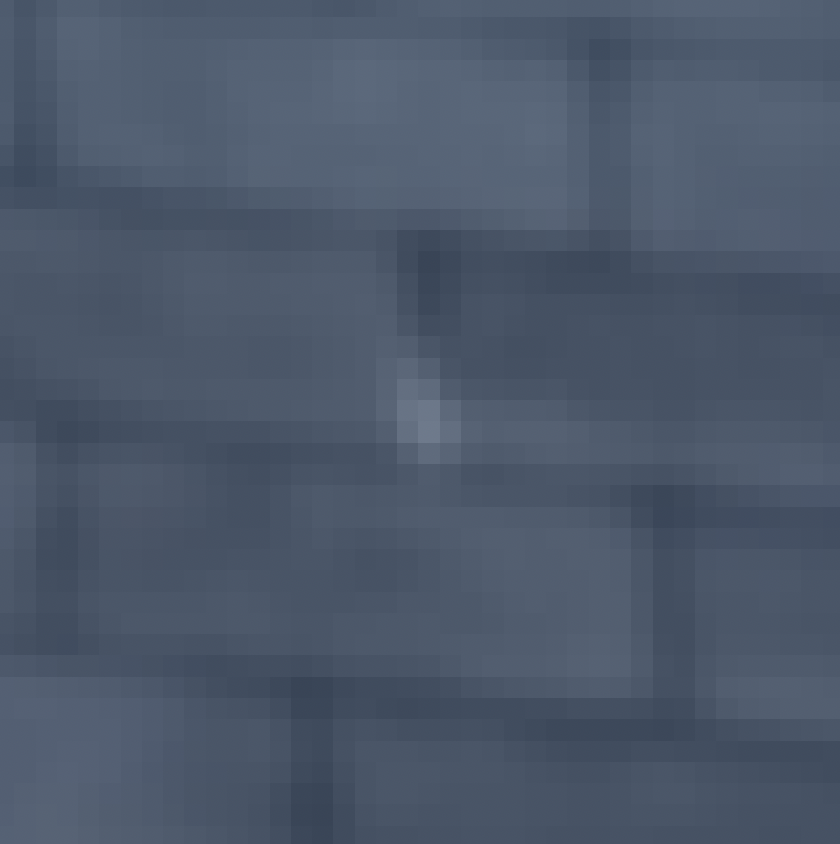


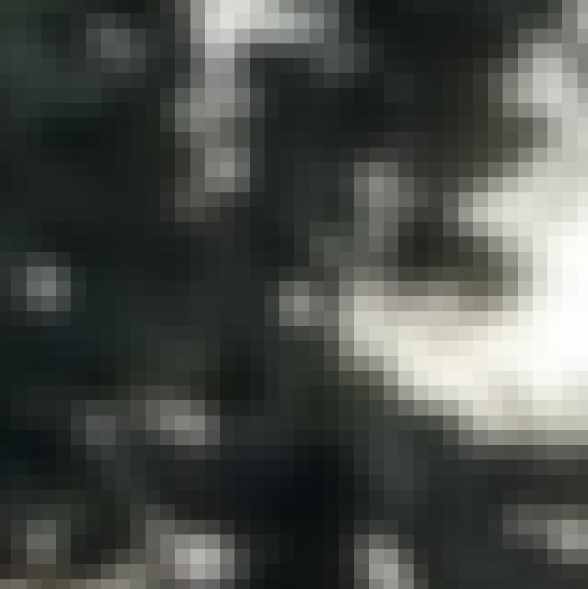


We will match 2 interest points that have similar features, and here we define "similarity" as the L2 distance between their feature patches. We could just match points to the point in the other image with the smallest distance, but this is prone to mistake. For example, an interest point's actual correspondence in the other image may not have been selected as a corner Harris or ANMS, or an interest point may have multiple matches in the other image due to repeating structures.
To reduce mistakes, we will use Lowe's technique, which works on the idea that if a feature truly matches, its nearest neighbor should be significantly closer (in terms of similarity) than its second-nearest neighbor. If the closest match is much better than the second-best match, this suggests that it's likely a true match. But if the closest match and the second-best match are very similar in distance, the match may be unreliable or ambiguous.
By only accepting matchings that have a significantly better nearest neighbor, we get the following matching:
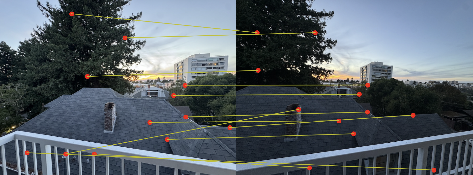
Note that some matchings in the railing area are incorrect because the repeating pattern makes it difficult to exactly match a corner. So Lowe's technique mitigates but does not fully resolve these mistakes.
We could build a homography using our current correspondances, but we could do better by computing the homography out of the "best of the best" correspondances. RANSAC is a method for only keeping the "inliers" in our group of correspondences. We loop over the following steps many times:
Lastly, we take the largest set of inliers we've ever seen as our final correspondences. Intuitively, the homography that yielded this largest set likely came from 4 accurate matchings, and so the inliers are likely accurate too.
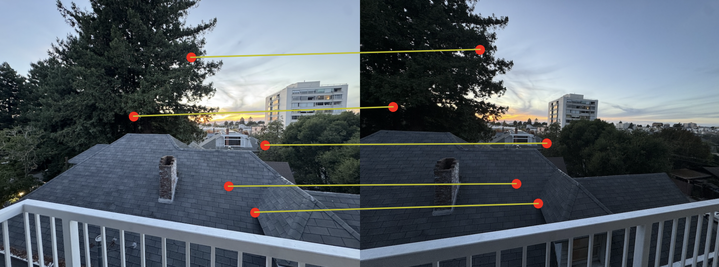
From here, we will use the same mosaic building algorithm as in the previous part! Let's compare the results:

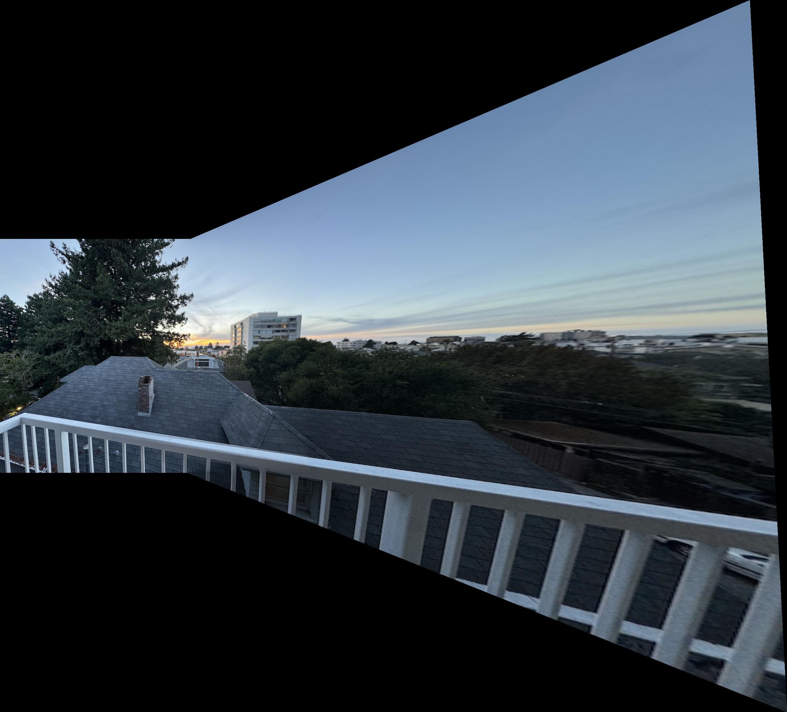
Both are very good, but the auto-stitched version actually has less skewing. This is very impressive, considering I had spent a lot of time manually selecting correspondences down to the best pixel.
The auto-stitched mosaics and the manual mosaics for living room and shoes are almost identical.

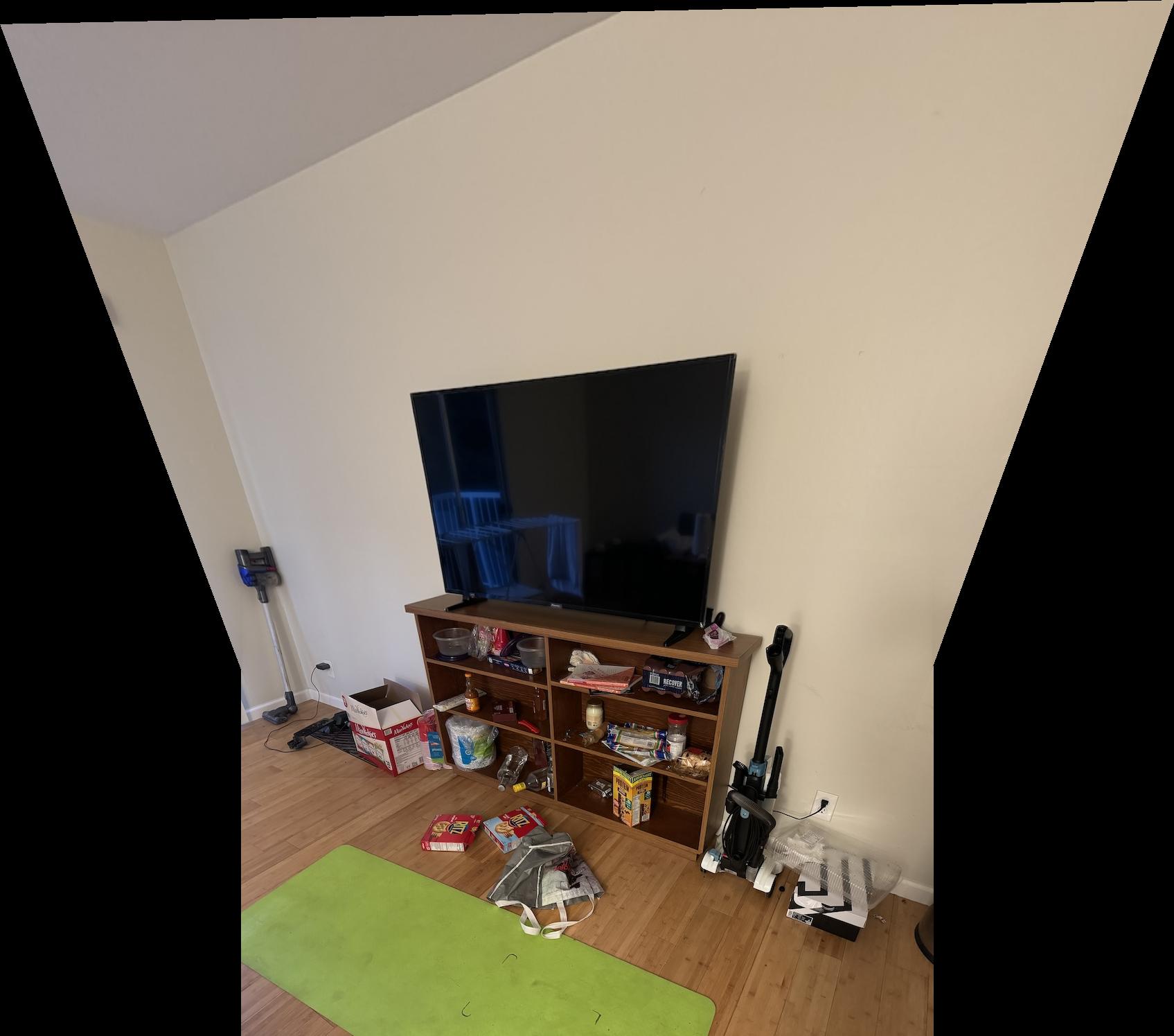

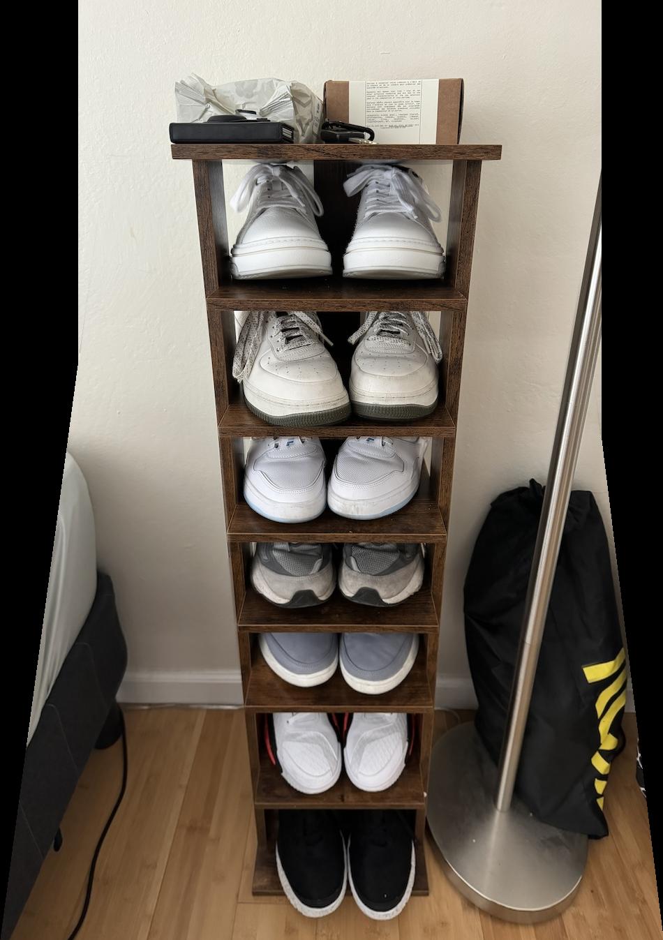
Some other auto-stitched mosaics I created.
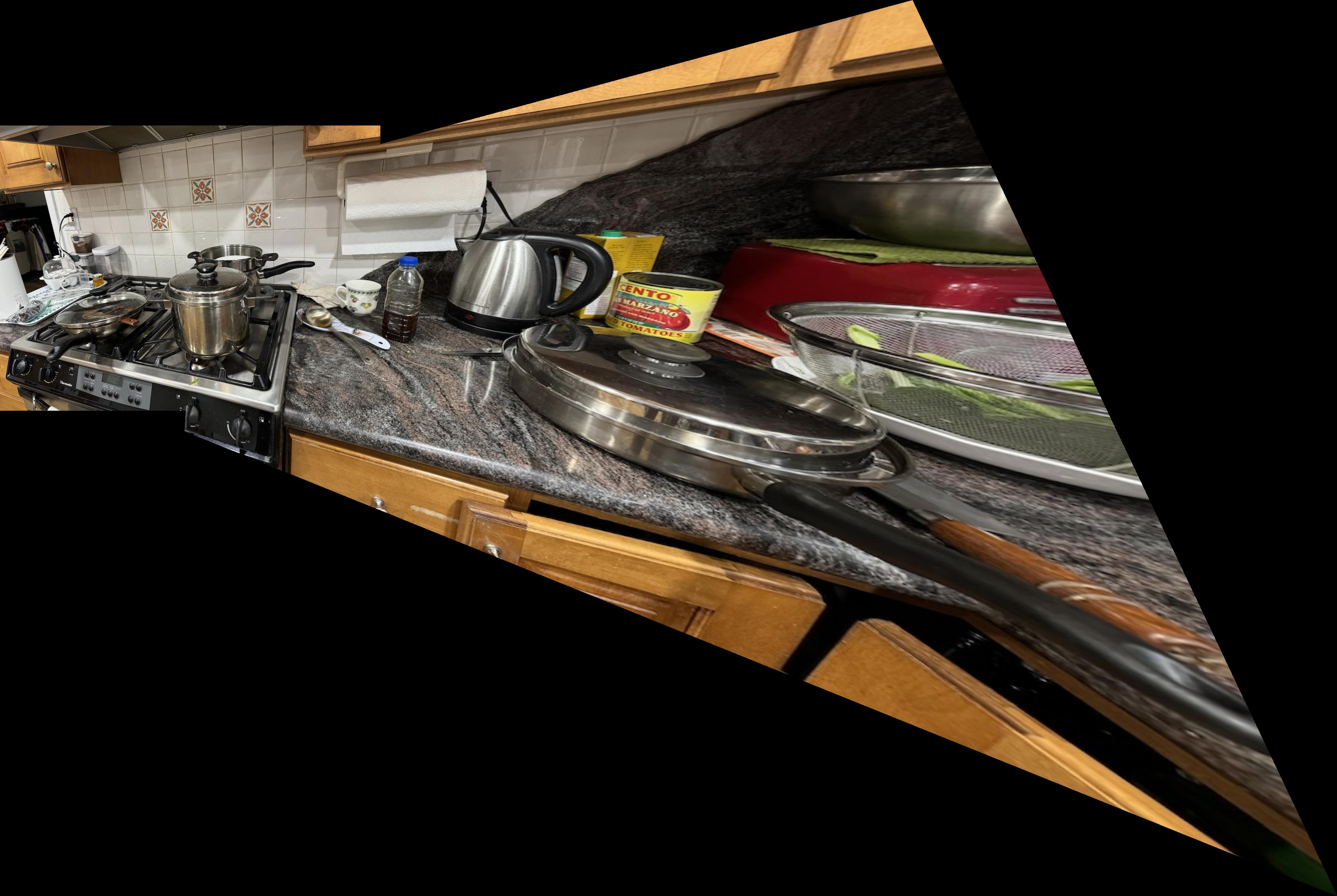
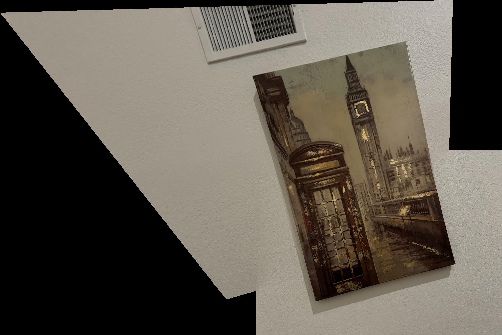
I really enjoyed the second part of the project because I could easily create mosaics without having to manually select a bunch of points! The most important thing I learned from this project is that having an intuitive understanding of why each step in an algorithm is important helps when implementing it. The automated feature matching algorithm consists of 5 relatively involved steps, so implementing each step at a time while keeping in mind the big picture allowed me to finish the project without much debugging.